
DEPRECATION NOTICE:
This blog post has since been accepted to the ICLR 2022 blog post track 🚀🚀. Check out https://iclr-blog-track.github.io/2022/03/25/ppo-implementation-details/ for the new improved blog post.
Deprecated Content:
The paper by Engstrom, Ilyas, et al. (https://arxiv.org/abs/2005.12729) points out that the code-level optimizations could be extremely important for the performance of Proximal Policy Optimization (PPO) algorithm. We (myself and Rousslan Dossa (https://github.com/dosssman)) have been spending the last several months trying to implement PPO to reproduce the reported results (https://arxiv.org/abs/1707.06347) on Atari and Mujoco.
Although Engstrom, Ilyas, et al. points out many code-level optimizations (9 in total), there are other implementation details that may have been left out (e.g. the use of vectorized environment or the way standard deviation is parameterized in continuous action space). In this blog post, we hope to compile a checklist of all implementation details of PPO with permanent links to the code.
Noticed that this blog post only lists out these details but does not provide ablation studies to examine the impact of these details. If you are interested in reading more, however, today I found out this paper (https://arxiv.org/pdf/2006.05990.pdf, submitted on 10 Jun 2020) that exactly provide empirical investigation on these details. Definitely a recommended read.
Important links before the main content
- Source code
- For Atari 2600 games:
- https://github.com/vwxyzjn/cleanrl/blob/master/cleanrl/ppo_atari.py
- https://github.com/vwxyzjn/cleanrl/blob/master/cleanrl/ppo_atari_visual.py (with action probability distribution visualization)
- For Mujoco, Pybullet and others:
- For Atari 2600 games:
- Our experiments metrics and videos of agents playing the game
Here the list goes in no particular order.
Note that each title of the trick has an permalink to where the trick is defined. As an example, 3. Normalization of Advantages corresponds to this Github Permalink: https://github.com/openai/baselines/blob/ea25b9e8b234e6ee1bca43083f8f3cf974143998/baselines/ppo2/model.py#L139
General implementation details
- Clipped surrogate objective
- Obviously, this is the core feature of PPO, so please implement it 😉.
- Generalized Advantage Estimation (GAE)
- Although the original PPO paper just uses the abstraction of advantage estimate in the PPO's objective, the implementation does use GAE.
- Normalization of Advantages
- After calculating the advantages based on GAE, the advantages vector is normalized by subtracting its mean and divided by its standard deviation. In particular, notice this normalization happens at the minibatch level instead of the whole batch level!
- Value Function Loss Clipping
- The value function loss is clipped in a manner that is similar to the PPO’s clipped surrogate objective.
- Overall Loss Includes Entropy Loss
- The overall loss is calculated as
loss = pg_loss - entropy * ent_coef + vf_loss * vf_coef, which includes entropy maximization, which intuitively encourages the exploration by encouraging the action probability distribution to be more chaotic.
- The overall loss is calculated as
- Adam Learning Rate Annealing
- The Adam optimizer’s learning rate could be either constant or set to decay. In particular, the hyper-parameters for training agents playing Atari games set the learning rate to decay from
2.5e-4to0as the number of timesteps agent trained increases. In mujoco, it decays from3e-4to0.
- The Adam optimizer’s learning rate could be either constant or set to decay. In particular, the hyper-parameters for training agents playing Atari games set the learning rate to decay from
- Mini-batch Updates
- The PPO implementation of the openai/baselines also uses mini-batches to compute the gradient and update the policy instead of the whole batch such as in openai/spinningup.
- Global Gradient Clipping
- For each update iteration in an epoch, the gradients of the policy and value network are clipped so that the “global l2 norm” (i.e. the norm of the concatenated gradients of all parameters) does not exceed
0.5
- For each update iteration in an epoch, the gradients of the policy and value network are clipped so that the “global l2 norm” (i.e. the norm of the concatenated gradients of all parameters) does not exceed
- Orthogonal Initialization of Weights and Constant Initialization of biases
- The related code is actually scattered all over the places in the openai/baselines library. The code to do such initialization is somehow in
baselines/baselines/a2c/utils.py, when in fact it is used for other algorithms such as PPO. In general, the weights of hidden layers use orthogonal initialization of weights with scalingnp.sqrt(2), and the biases are set to0, as shown in the CNN initialization for Atari, and the MLP initialization for Mujoco, which are located atbaselines/baselines/common/models.py. However, the weights of the policy output layer are initialized with the scale of0.01, and the weights of the value output layer are initialized with the scale of1, and their corresponding code is located atbaselines/baselines/common/policies.py. By the way, it seems the implementation of the orthogonal initialization of openai/baselines seems different from that of pytorch/pytorch, but I consider this to be a very low-level detail that should not have much impact on the performance.
- The related code is actually scattered all over the places in the openai/baselines library. The code to do such initialization is somehow in
- The Use of Parallelized Environment
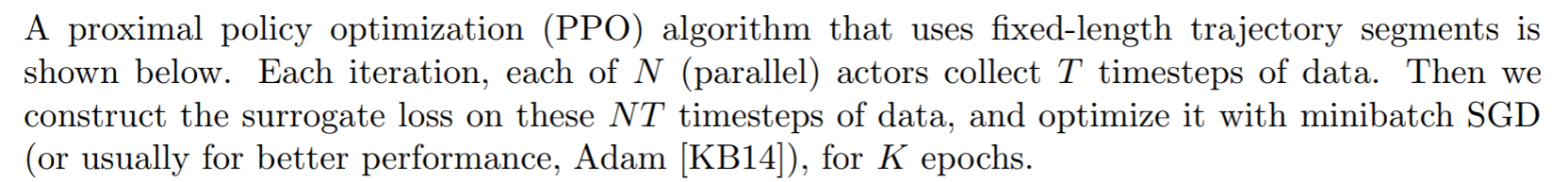
- PPO uses the parallelized environment to speed up execution. As mentioned in the paper, it uses ``fixed-length trajectory segments''. I think the use of such environments is actually under-appreciated by most people, as it kind of changes the underlying MDP somehow. I will dedicate a section below to discuss it in detail.
- The Epsilon Parameter of Adam Optimizer
- By default, this parameter is not in the list of configurable hyper-parameters of PPO. However, it is set to
1e-5, Which is different than the default epsilon of1e-8in PyTorch and TensorFlow.
- By default, this parameter is not in the list of configurable hyper-parameters of PPO. However, it is set to
Mujoco specific implementation details
# https://github.com/openai/baselines/blob/master/baselines/ppo2/defaults.py
def mujoco():
    return dict(
        nsteps=2048,
        nminibatches=32,
        lam=0.95,
        gamma=0.99,
        noptepochs=10,
        log_interval=1,
        ent_coef=0.0,
        lr=lambda f: 3e-4 * f,
        cliprange=0.2,
        value_network='copy'
    )
The hyper-parameters of Mujoco related experiments are listed above, and here are some important details mostly related to the use of the normalization wrappers. Specifically, when you run commands such as python -m baselines.run --alg=ppo2 --env=Humanoid-v2 --network=mlp --num_timesteps=2e7, you are using baselines/baselines/run.py In particular, when the environment is of type Mujoco, the run.py applies the VecNormalize wrapper to the environment, as shown here.
- Normalization of Observation
- At each timestep, the
VecNormalizewrapper pre-processes the observation before feeding it to the PPO agent. The raw observation was normalized by subtracting its running mean and divided by its variance.
- At each timestep, the
- Observation Clipping
- Followed by the normalization of observation, the normalized observation is further clipped by
VecNormalizeto a range, usually [−10, 10].
- Followed by the normalization of observation, the normalized observation is further clipped by
- Reward Scaling
- The
VecNormalizealso applies a certain discount-based scaling scheme, where the rewards are divided by the standard deviation of a rolling discounted sum of the rewards (without subtracting and re-adding the mean).
- The
- Reward Clipping
- Followed by the scaling of reward, the scaled reward is further clipped by
VecNormalizeto a range, usually [−10, 10].
- Followed by the scaling of reward, the scaled reward is further clipped by
- The Way Standard Deviation is Paramterized
- Policy gradient methods (including PPO) assume the continuous actions are sampled from a normal distribution. So to create such distribution, the neural network needs to output the mean and standard deviation of the continuous action. The implementation outputs the logits for the mean, but instead of outputting the logits for the standard deviation, it outputs the logarithm of the standard deviation. In addition, this
log stdis set to be state-independent and initialized to be 0.
- Policy gradient methods (including PPO) assume the continuous actions are sampled from a normal distribution. So to create such distribution, the neural network needs to output the mean and standard deviation of the continuous action. The implementation outputs the logits for the mean, but instead of outputting the logits for the standard deviation, it outputs the logarithm of the standard deviation. In addition, this
- Hyperbolic Tangent Activations
- The activation functions of the hidden layers are always set to use the hyperbolic tangent function.
- Not Sharing Hidden Layers for Policy and Value Functions
- The network of the policy and value functions are initialized separately.
- Handling of action clipping to valid range and storage
- After a continuous action is sampled, Such action could be invalid because it could exceed the valid range of continuous actions in the environment. To avoid this, add applies the rapper to clip the action into the valid range. However, the original unclipped action is stored as part of the episodic data.
Atari specific implementation details
# https://github.com/openai/baselines/blob/master/baselines/ppo2/defaults.py
def atari():
    return dict(
        nsteps=128, nminibatches=4,
        lam=0.95, gamma=0.99, noptepochs=4, log_interval=1,
        ent_coef=.01,
        lr=lambda f : f * 2.5e-4,
        cliprange=0.1,
    )
The hyperparameters of Atari-related experiments are listed above. Similarly, atari wrappers are applied when calling baselines/baselines/run.py. For more information on the atari wrappers, see how this is done in the DQN paper (https://www.cs.toronto.edu/~vmnih/docs/dqn.pdf).
- The Use of
NoopResetEnv- This wrapper samples initial states by taking a random number of no-ops on reset. No-op is assumed to be action 0.
- The Use of
FireResetEnv- This wrapper takes action of
FIREon reset for environments that are fixed until firing.
- This wrapper takes action of
- The Use of
EpisodicLifeEnv- This wrapper makes end-of-life == end-of-episode but only resets on the true game over. Done by DeepMind for the DQN and co. since it helps value estimation. This is an arguably very interesting wrapper in my opinion because it changes the initial state distribution of the game.
- The Use of
MaxAndSkipEnv- This wrapper repeats actions, sums rewards, and returns the max-pooled observation.
- The Use of
WarpFrame- This wrapper warps frames to 84x84 as done in the Nature paper and later work. If the environment uses dictionary observations
- The Use of
FrameStack- This wrapper stacks k last frames such that the agent can infer the velocity and directions of moving objects.
- The Use of
ClipRewardEnv- This wrapper bins reward to {+1, 0, -1} by its sign. According to our initial experiments, it seems to have a huge impact on the PPO's performance on Breakout.
- Scaling the Images to Range [0, 1]
- The input data has the range of [0,255], but it is divided by 255 to be in the range of [0,1]. My initial experiments found this scaling to be extremely important. Without it, the first policy update results in the Kullback–Leibler divergence explodes, likely due to how the layers are initialized.
- Rectified Linear Unit (ReLU) Activations
- The activation functions for the hidden and output layers are always ReLU.
- Sharing Hidden Layers for Policy and Value Functions
- The hidden layers for the policy and value functions share the same weights and biases. Although I don't think it makes much difference for the performance, the computational cost is definitely reduced since only one set of hidden layers needs to be optimized.
Auxiliary implementation details
- Clip Range Annealing
- The clip coefficient of PPO can be annealed similar to how the learning rate is annealed. However, as shown by the hyperparameters above, the clip range annealing is actually not used.
- Parallellized Gradient Update
- The policy gradient is calculated in parallel using multiple processes. However, I consider this as an auxiliary detail because it is difficult to implement and according to my experience does not improve the performance, measured in episode rewards achieved.
- Early Stopping
- This is not actually an implementation detail of openai/baselines, but rather an implementation detail in openai/spinningup. This early stopping optimization measures that mean KL divergence between the target and the current policy of PPO, and stops the policy updates of the current epoch if the mean KL divergence exceeds some preset threshold. This feature is implemented and can be toggled by using
--kle-stop
- This is not actually an implementation detail of openai/baselines, but rather an implementation detail in openai/spinningup. This early stopping optimization measures that mean KL divergence between the target and the current policy of PPO, and stops the policy updates of the current epoch if the mean KL divergence exceeds some preset threshold. This feature is implemented and can be toggled by using
A dedicated note to the use of parallelized environment
As mentioned in the paper, it uses ``fixed-length trajectory segments'' as shown by the screenshot below, but what does that even mean?
To really understand its impact, it's important to understand how an episode of the game could terminate. In general, there are two termination models: true termination and time limit termination.
- True termination. The episode of the game really terminates. As an example, the true termination of the Breakout game in Atari 2600 comes when you lose all of your lives.
- Time limit termination. To avoid the episode of the game going on indefinitely, the episode of the game is set to finish with a maximum of N time steps.
To illustrate, let's first consider a toy game environment TestEnv that always outputs its observation as its current time step from t=0, and always truly terminates at t=10.
import gym
import numpy as np
from gym import error, spaces, utils
from gym.envs.registration import register

"""
First kind of termination: true termination
As an example, the true termination of the Breakout game in Atari 2600
comes when you lose all of your lives.
"""
class TestEnv(gym.Env):
    """
    A simple env that always ends after 10 timesteps, which
    can be considered as the ``true termination'' from the environment.
    At each timestep, its observation is its internal timestep
    """
    def __init__(self):
        self.action_space = spaces.Discrete(2)
        self.observation_space = spaces.Box(low=np.array([-1.]),
            high=np.array([10.]))
    def step(self, action):
        self.t += 1
        return np.array([0.])+self.t, 1, self.t==10, {}
    def reset(self):
        self.t = 0
        return np.array([0.])+self.t

if "TestEnv-v0" not in gym.envs.registry.env_specs:
    register(
        "TestEnv-v0",
        entry_point='__main__:TestEnv'
    )

env = gym.make("TestEnv-v0")
print(f"env is {env}")
for i in range(2):
    all_obs = [env.reset()]
    while True:
        obs, reward, done, info = env.step(env.action_space.sample())
        all_obs += [obs]
        if done:
            print(f"all observation in episode {i}:")
            print(all_obs)
            print("true termination")
            print()
            break
print("=========")
env is <TestEnv<TestEnv-v0>>
all observation in episode 0:
[array([0.]), array([1.]), array([2.]), array([3.]), array([4.]),
array([5.]), array([6.]), array([7.]), array([8.]), array([9.]), array([10.])]
true termination
all observation in episode 1:
[array([0.]), array([1.]), array([2.]), array([3.]), array([4.]),
array([5.]), array([6.]), array([7.]), array([8.]), array([9.]), array([10.])]
true termination
=========As shown above, the episodic observations of both episodes are the same and of the same length H=11 (H stands for horizon). However, in real games, this H could get arbitrarily large, which could be very undesirable if you want to collect a finite number of observations to train agents. To avoid an episode that never finishes, we typically put a time limit on the episode length. In the implementation, this is achieved by using the gym.wrappers.TimeLimit wrapper.
"""
Second kind of termination: TimeLimit termination
As an example, TimeLimit termination comes when the episode of "CartPole-v0"
exceeds length 200.
"""
if "TestEnvTimeLimit3-v0" not in gym.envs.registry.env_specs:
    register(
        "TestEnvTimeLimit3-v0",
        entry_point='__main__:TestEnv',
        max_episode_steps=8
    )

env = gym.make("TestEnvTimeLimit3-v0")
# equivalent to below
# env = TestEnv()
# env = gym.wrappers.TimeLimit(env, max_episode_steps=8)
print(f"env is {env}")
print(f"env's timelimit is {env._max_episode_steps}")
for i in range(2):
    all_obs = [env.reset()]
    while True:
        obs, reward, done, info = env.step(env.action_space.sample())
        all_obs += [obs]
        if done:
            print(f"all observation in episode {i}:")
            print(all_obs)
            print("TimeLimit termination")
            print()
            break
print("=========")
env is <TimeLimit<TestEnv<TestEnvTimeLimit3-v0>>>
env's timelimit is 8
all observation in episode 0:
[array([0.]), array([1.]), array([2.]), array([3.]), array([4.]),
array([5.]), array([6.]), array([7.]), array([8.])]
time limit termination
all observation in episode 1:
[array([0.]), array([1.]), array([2.]), array([3.]), array([4.]),
array([5.]), array([6.]), array([7.]), array([8.])]
time limit termination
=========That's shown above, the gym.wrappers.TimeLimit wrapper makes the environment always terminate at t=8. Well, the problem is that some games need to have extremely large time limits to make sense. As an example, a game of Dota 2 could last for millions of times steps. How do we handle all these observations without blowing up our memory? This is where the parallelized environment VecEnv comes in, it reduces the episodic observations to ``fixed-length trajectory segments'', which introduces the third type of episodic termination:
Early termination induced by fixed trajectory.
Here is an example
from stable_baselines3.common.vec_env import DummyVecEnv
"""
Third kind of termination: early termination induced by fixed
trajectory length of `n_steps`
This is usually combined with TimeLimit wrapped env,
but you can use it without the TimeLimit
"""
n_steps = 5
envs = DummyVecEnv([
    lambda: gym.make("TestEnvTimeLimit3-v0")])
print(f"envs is {envs}")
print(f"envs' timelimit is {envs.envs[0]._max_episode_steps}")
obss = envs.reset()
for i in range(3):
    all_obss = []
    for j in range(n_steps):
        all_obss += [obss.astype("float")]
        obss, rewards, dones, infos = envs.step(np.array([1.,1.]))
        # print(infos)

    print(f"all observation in trajectory {i}:")
    print(all_obss)
    print("early termination by `n_steps`")
    print()
print("=========")
envs is <stable_baselines3.common.vec_env.dummy_vec_env.DummyVecEnv
object at 0x7f7381256f10>
envs' timelimit is 8
all observation in trajectory 0:
[array([[0.]]), array([[1.]]), array([[2.]]), array([[3.]]), array([[4.]])]
early termination by `n_steps`
all observation in trajectory 1:
[array([[5.]]), array([[6.]]), array([[7.]]), array([[0.]]), array([[1.]])]
early termination by `n_steps`
all observation in trajectory 2:
[array([[2.]]), array([[3.]]), array([[4.]]), array([[5.]]), array([[6.]])]
early termination by `n_steps`
=========What's really interesting is the observation data in the second trajectory (trajectory 1). We offer some observations.
- The initial observation of the trajectory is no longer always
array([0.]), which means the initial state distribution of the trajectory is no longer the same as that of the original MDP. - The time-limited episode of the game is broken into pieces presented in different trajectories.
- The terminal observation
array([8.])is not present in any trajectory.
The benefit is obvious: the usage of parallelized environment allows PPO to handle games with arbitrarily long horizons. By carefully using storing variables dones and using value bootstrapping, it is possible to still calculate advantages and returns to update the agents, as it is done here. However, notice openai/baselines only bootstrap values if the trajectory is terminated due to Early termination, but provide no value bootstraps if time limit termination happens.
Results
I think it's important to benchmark our implementation against a variety of different games to ensure quality. A lot of the implementations that I've seen are usually only tested with one specific game, and when trying to run these implementations with other games they often fail.
We now present our results on atari 2600 and MuJoCo games, which matches the published results quite well. You may also find detailed experiment logging, various running metrics, and videos of agents playing the game in https://app.wandb.ai/cleanrl/cleanrl.benchmark/reports/PPO-Reproduction--VmlldzoxMzAzNTQ
Results on Atari


Results on Mujoco


Results on Pybullet and others


A case study on HalfCheetah-v2
The performance of PPO on is suspiciously low (only about 1500 for episode reward) on HalfCheetah-v2 as I have had a PPO implementation with better performance in this environment. So I decided to run openai/baselines's PPO on this environment to see if my implementation and will have a different performance. Fortunately, The performance is exactly the same.

Additionally, by examining the videos of the agents actually playing the game, We get a sense of why the performance is sub optimal, which is quite frankly hilarious, where the agent learns to move by using its head. This highlights why you need the videos of agents playing the game to develop better understanding of the agents behavior. This video is downloaded at https://app.wandb.ai/cleanrl/cleanrl.benchmark/runs/3cth77iq?workspace=user-costa-huang
Fun visualization of action probability distribution
The videos of agents playing the game are recorded through the gym.wrappers.Monitor wrapper, which records the videos based on the image numpy array produced by the env.render(mode="rgb_array") method. So by overriding this method, we can actually visualize the action probability distribution and let it be recorded through a simple wrapper. And below is an example of our visualization of the action probability distribution of agents playing Breakout.
Calling env.unwrapped.get_action_meanings() suggests the four colors mean actions ['NOOP', 'FIRE', 'RIGHT', 'LEFT'], downloaded here https://app.wandb.ai/cleanrl/cleanrl.benchmark/runs/thq5rgnz?workspace=user-costa-huang.
Reproduction of our results
Since we use Weights and Biases to record the experiments, you first need to get register an account and get an API key. Then, one of the easiest ways to reproduce our results is to run commands similar to the following.
wandb login

for seed in {1..2}
do
    (sleep 0.3 && nohup xvfb-run -a python ppo_atari_visual.py \
    --gym-id BeamRiderNoFrameskip-v4 \
    --total-timesteps 10000000 \
    --wandb-project-name cleanrl.benchmark \
    --wandb-entity cleanrl \
    --prod-mode \
    --capture-video \
    --seed $seed
    ) >& /dev/null &
done

for seed in {1..2}
do
    (sleep 0.3 && nohup xvfb-run -a python ppo_continuous_action.py \
    --gym-id Hopper-v2 \
    --total-timesteps 2000000 \
    --wandb-project-name cleanrl.benchmark \
    --wandb-entity cleanrl \
    --prod-mode \
    --capture-video \
    --seed $seed
    ) >& /dev/null &
done
The full list of these commands can be found at https://gist.github.com/vwxyzjn/2d66ff396741e5b9038012a1deb48062#file-ppo-sh
An alternative way that is also easy is to use docker containers by running commands similar to the following
docker run -d --cpuset-cpus="0" -e WANDB={REPLACE_WITH_YOUR_WANDB_KEY} \
 vwxyzjn/cleanrl:latest python ppo_atari_visual.py \
--gym-id BeamRiderNoFrameskip-v4 --total-timesteps 10000000 \
--wandb-project-name cleanrl.benchmark --wandb-entity cleanrl \
--prod-mode --capture-video --seed 1
The full list of these commands can be found at https://gist.github.com/vwxyzjn/2d66ff396741e5b9038012a1deb48062#file-docker-sh, unfortunately, we do not have docker commands for Mujoco environments because my student license cannot be used in a docker container.
About our CleanRL
This work is done using some very common code structures found in CleanRL. In CleanRL, we try to create high-quality single file implementation of deep reinforcement learning algorithms with many research-friendly features.
Research-friendly features
- Seeding of everything
- Our implementation always has a section the seeds the following modules. Although there are still sources of indeterminism for some environments, results are mostly reproducible within a single machine. This makes debugging a lot easier.
- Cloud experiment management
- We use a cloud experiment management service named weights and biases. It logs the hyperparameters, training metrics (e.g. episode reward, training losses), system metrics (e.g. CPU utilization, memory utilization),
stdout, stderr, source code (this is especially helpful since we have single file implementation, which makes version management very easy), and videos of the agents playing games.
- We use a cloud experiment management service named weights and biases. It logs the hyperparameters, training metrics (e.g. episode reward, training losses), system metrics (e.g. CPU utilization, memory utilization),
- Cloud video logging of agents playing the game
- I want to additionally stress the importance of logging the videos of the agents playing games. Visually inspected the agents' actual behavior gives you far more insight than the metric of episode reward could ever give you.
- Integration with Docker and AWS Batch
- CleanRL actually scales quite well if your experiments individually don't run for billions of time steps. We package the files into docker containers, and by leveraging AWS batch, we have finished tasks about 8000 CPU-hours in four hours, costing about $100 via spot instances. One of those days I'll find time to write instructions on how to do that 😅.
- For now, just know you can run experiments using
docker run -d --cpuset-cpus="1" -e WANDB=xxxxxxxxxxxxxxxxxxxxxxxxxxxxxxxx vwxyzjn/cleanrl:latest python ppo_atari_visual.py --gym-id BreakoutNoFrameskip-v4 --total-timesteps 10000000 --wandb-project-name cleanrl.benchmark --wandb-entity cleanrl --prod-mode --capture-video --seed 2
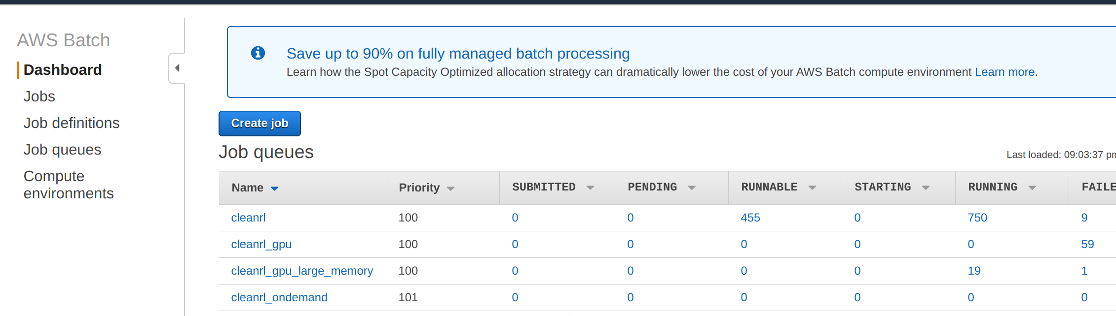
Running thousands of experiments using docker and aws batch
Long-term goal: Open RL Benchmark
Our long-term goal is to create an open RL benchmark that is easy to examine and reproduce. You can already see a prototype of such benchmark at http://cleanrl.costa.sh. Our use of Weights and Biases transforms a static image to something much greater that allows the researcher to examine many important metrics, visually inspect the trained agents playing the game, and obtain all information needed to reproduce the results, as shown in the video below.
You should be able to just download the code, and run the command in the Overview page to reproduce this particular run!
I see its great potential in not only bringing the transparency of RL implementation to a whole new level but also accelerating research because the reproduction of these algorithms becomes trivially easy and readily accessible.
Getting involved
Our monthly development cycle. If you're interested in our work and share our passion to create high-quality single file implementation of deep reinforcement learning algorithms with many research-friendly features, please consider joining us at Discord. Each month, we usually set up a development plan to reproduce a paper. Then in each week, we have online meetings to discuss the literature and implementation of the algorithms presented in the paper. All of our previous meetings are recorded on YouTube, and we have had 21 meetings at the time of this writing.
Getting supports. If you have any questions regarding our implementations, Feel free to raise a GitHub issue or directly asking us on the discord.
Support us
If you enjoy this intellectual effort and it really has helped you research, you should consider support me on Github Sponsors or Rousslan (who is also a main contributor) here. Your contribution will be much appreciated and likely be used to buy coffee or computational resources on AWS. But more importantly, your contribution will inspire us to create more work like this to reproduce the state of the art results.
I hope you enjoy reading this blog post very much. If you have any questions, feel free to comment down below.